A small population of unicellular organisms presented with abundant resources and ample space will increase exponentially (Figure 6.1a). Population doubling time T_d (hours or days) is a function of an inherent capacity for cell division and enlargement which is expressed according to environmental conditions. In Figure 6.1(a) doubling times for these two populations are 1 and 2 d for fast and slow strains respectively.

Exponential curves such as those in Figure 6.1(a) are described mathematically as

\[N(t)=N_0e^{rt} \tag{6.1}\]

 where N(t) is the number of cells present at time t, N₀ is the population at time 0, r determines the rate at which the population grows, and e is the base of the natural logarithm. By derivation from Equation 6.1

\[r=\frac{1}{N}\frac{\text{d}N(t)}{\text{d}t} \tag{6.2}\]

and is called relative growth rate with units of 1/time. The doubling time is T_d = (ln 2)/r.

If a population or an organism has a constant relative growth rate then doubling time is also constant, and that population must be growing at an exponential rate given by Equation 6.1. The ‘fast’ strain in Figure 6.1(a) is doubling every day whereas the ‘slow’ strain doubles every 2 d, thus r is 0.69 d^–1 and 0.35 d^–1, respectively.

If cell growth data in Figure 6.1(a) are converted to natural logarithms (i.e. ln transformed), two straight lines with contrasting slopes will result (Figure 6.1b). For strict exponential growth where N(t) is given by Equation 6.1,

 \[\text{ln }N(t)=\text{ln }N_0+rt\tag{6.3}\]

 which is the familiar slope-intercept form of a linear equation, so that a plot of ln N(t) as a function of time t is a straight line whose slope is relative growth rate r, and intercept is ln N₀

In practice, r is inferred by assessing cell numbers N₁ and N₂ on two occasions, t₁ and t₂ (separated by hours or days depending on doubling time — most commonly days in plant cell cultures), and substituting those values into the expression

\[r=\frac{\text{ln }N_2-\text{ln }N_1}{t_2-t_1}\tag{6.4}\]

which expresses r in terms of population numbers N₁ and N₂ at times t₁ and t₂, respectively.

If growth is exponential, Eq. 6.3 will be linear and any two time points and the natural logarithm of their corresponding population sizes will give an estimate of the growth rate, r. However, if relative growth rate r is not constant, then growth is not exponential but the concept of relative growth rate is still useful for analysis of growth dynamics in populations or organisms. Equation 6.3 is then used to compute average relative growth rate between times t₁ and t₂ even though population growth might not follow Equation 6.1 in strict terms. In that case plots analogous to Figure 6.1(b) will not be straight lines.

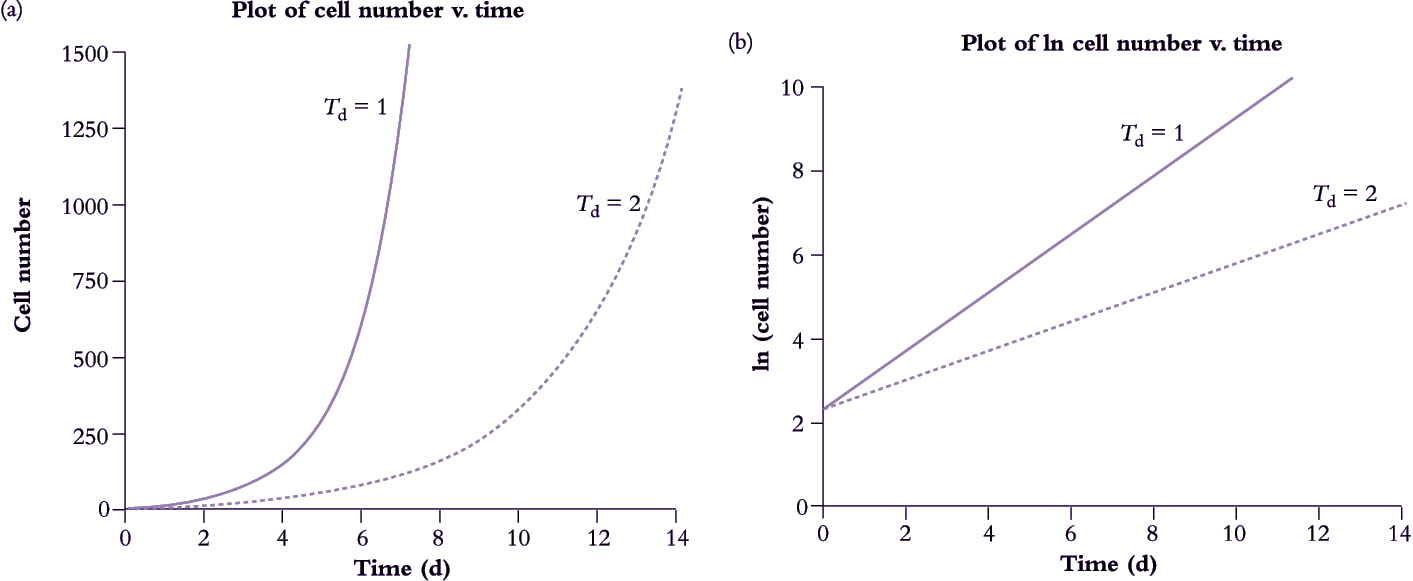
In whole plants, cell number is an impractical measure of growth. Instead, fresh or oven-dried biomass (W) is generally taken as a surrogate for cell growth and referenced to the number of days elapsed between successive observations. Relative growth rate is now known as RGR rather than r and measured in days or weeks rather than hours.

Relative growth rate, RGR (d^–1), can be expressed in terms of differential calculus as \(RGR=\frac{1}{W}\frac{\text{d}W}{\text{d}t}\) (compare Equation 6.2.) so that RGR is increment in dry mass (dW) per increment in time (dt) divided by existing biomass (W). Averaged over a time interval t₁ to t₂ during which time biomass increases from W₁ to W₂, RGR (d^–1) can be calculated from

\[\text{RGR}=\frac{\text{ln }W_2-\text{ln } W_1}{t_2-t_1} \tag{6.5} \]

which is analogous to Eq, 6.4. Net gain in biomass (W) is the outcome of CO₂ assimilation by leaves minus respiratory loss by the entire plant. Leaf area can therefore be viewed as a driving variable, and biomass increment (dW) per unit time (dt) can then be divided by leaf area (A) to yield the net assimilation rate, NAR (g m^–2 d^–1), where

\[\text{NAR}=\frac{1}{A}\frac{\text{d}W}{\text{d}T} \tag{6.6}\]

Averaged over a short time interval (t₁ to t₂ days) and provided whole-plant biomass and leaf area are linearly related (see Radford 1967),

\[\text{NAR}=\left(\frac{W_2-W_1}{t_2-t_1}\right)\left(\frac{\text{ln }A_2-\text{ln }A_1}{A_2-A_1}\right) \tag{6.7}\]

NAR thus represents a plant’s net photosynthetic effectiveness in capturing light, assimilating CO₂ and storing photoassimilate. Variation in NAR can derive from differences in canopy architecture and light interception, photosynthetic activity of leaves, respiration, transport of photoassimilate and storage capacity of sinks, or even the chemical nature of stored products.

The following treatment assumes for simplicity that photosynthesis and the assimilation of CO₂ occurs only in leaves, even though for many herbaceous or succulent species it occurs to a lesser degree also in stems. Since leaf area is a driving variable for whole-plant growth, the proportion of plant biomass invested in leaf area will have an important bearing on RGR, and can be conveniently defined as leaf area ratio, LAR (m² g^–1), where

\[\text{LAR}=\frac{A}{W}\tag{6.8}\]

LAR can be factored into two components: specific leaf area (SLA) and leaf weight ratio (LWR). SLA is the ratio of leaf area (A) to leaf mass (W_L) (m² g^–1) and LWR is the ratio of leaf mass (W_L) to total plant mass (W) (dimensionless). Thus,

\[\begin{align} \text{LAR} &=  \frac{A}{W_L}\frac{W_L}{W} \\
 &=  \text{SLA} \times \text{LWR} \end{align} \tag{6.9} \]

As an aside, average LAR over the growth interval t₁ to t₂ is

 \[\text{LAR}=\frac{1}{2} \left( \frac{A_1}{W_1}+\frac{A_2}{W_2} \right) \tag{6.10}\]

Expressed this way, LAR becomes a more meaningful growth index than A/W (Equation 6.8) and can help resolve sources of variation in RGR.

If both A and W are increasing exponentially so that W is proportional to A, it follows that

\[\frac{1}{W}\frac{\text{d}W}{\text{d}t}=\frac{1}{A}\frac{\text{d}W}{\text{d}t}\times\frac{A}{W}\tag{6.11}\]

0r (substituting Equations 6.5, 6.6 and 6.8)

\[\text{RGR}=\text{NAR}\times \text{LAR} \tag{6.12}\]

As LAR can be broken into SLA and LWR (Equation 6.9) then

\[\text{RGR}=\text{NAR}\times \text{LWR} \times \text{SLA} \tag{6.13}\]

Sources of variation in RGR partitioned this way provide useful insights on driving variables in process physiology and ecology. For an expanded discussion on methodological issues associated with the determination of RGR in experimental populations see Poorter and Lewis (1986).

Increases in leaf area over time can be a more useful basis for measuring plant growth rates than biomass increases, particularly as non-destructive techniques for measuring leaf area are now available. Plant growth rate can be measured as the relative increase in leaf area over time, by substituting total plant leaf area for total biomass in the conventional RGR equation.

\[\text{RGR}_\text{A} =\frac{\text{ln } LA_2 - \text{ln } LA_1}{t_2-t_1} \tag{6.14} \]

where RGR_A is relative leaf area expansion rate, LA is total plant leaf area and t is time at two time intervals, t₁ and t₂, preferably 2-3 days apart.

Growth indices in summary

Five key indices are commonly derived as an aid to understanding growth responses. Mathematical and functional definitions of those terms are summarised below.

Growth index	Mathematical definition	Units	Functional definition
Relative growth rate RGR	\(\frac{1}{W}\frac{\text{d}W}{\text{d}t}\)	d-1	Rate of mass increase per unit mass present (efficiency of growth with respect to biomass)
Net assimilation rate NAR	\(\frac{1}{A}\frac{\text{d}W}{\text{d}t}\)	g m-2 d-1	Rate of mass increase per unit leaf area (efficiency of leaves in generating biomass)
Leaf area ratio LAR	\(\frac{A}{W}\)	m2 g-1	Ratio of leaf area to total plant mass (a measure of ‘leafiness’ or photosynthetic area relative to respiratory mass)
Specific leaf area SLA	\(\frac{A}{W_L}\)	m2 g-1	Ratio of leaf area to leaf mass (a measure of thickness of leaves relative to area)
Leaf weight ratio LWR	\(\frac{W_L}{W}\)	dimension-less	Ratio of leaf mass to total plant mass (a measure of biomass allocation to leaves)