6.1.1 - Cell populations

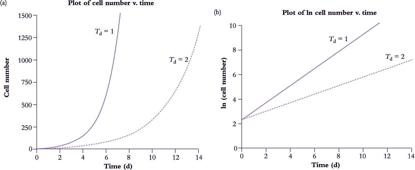
A small population of unicellular organisms presented with abundant resources and ample space will increase exponentially (Figure 6.1a). Population doubling time T_d (hours or days) is a function of an inherent capacity for cell division and enlargement which is expressed according to environmental conditions. In Figure 6.1(a) doubling times for these two populations are 1 and 2 d for fast and slow strains respectively.

Fig 6.1.png

Figure 6.1. A population of cells unrestricted by space or substrate supply will grow exponentially. In this hypothetical case, a fast-growing strain of a single-celled organism with a doubling time of 1 d starts on day 0 with a population of n cells which increases to 120·n by day 7. In this example, n=10. The slow-growing strain with a doubling time of 2 d takes twice as long to reach that same size. When data for cell numbers are ln transformed, exponential curves (a) become straight lines (b) where slope = r.

Exponential curves such as those in Figure 6.1(a) are described mathematically as

\[N(t)=N_0e^{rt} \tag{6.1}\]

 where N(t) is the number of cells present at time t, N₀ is the population at time 0, r determines the rate at which the population grows, and e is the base of the natural logarithm. By derivation from Equation 6.1

\[r=\frac{1}{N}\frac{\text{d}N(t)}{\text{d}t} \tag{6.2}\]

and is called relative growth rate with units of 1/time. The doubling time is T_d = (ln 2)/r.

If a population or an organism has a constant relative growth rate then doubling time is also constant, and that population must be growing at an exponential rate given by Equation 6.1. The ‘fast’ strain in Figure 6.1(a) is doubling every day whereas the ‘slow’ strain doubles every 2 d, thus r is 0.69 d^–1 and 0.35 d^–1, respectively.

If cell growth data in Figure 6.1(a) are converted to natural logarithms (i.e. ln transformed), two straight lines with contrasting slopes will result (Figure 6.1b). For strict exponential growth where N(t) is given by Equation 6.1,

 \[\text{ln }N(t)=\text{ln }N_0+rt\tag{6.3}\]

 which is the familiar slope-intercept form of a linear equation, so that a plot of ln N(t) as a function of time t is a straight line whose slope is relative growth rate r, and intercept is ln N₀

In practice, r is inferred by assessing cell numbers N₁ and N₂ on two occasions, t₁ and t₂ (separated by hours or days depending on doubling time — most commonly days in plant cell cultures), and substituting those values into the expression

\[r=\frac{\text{ln }N_2-\text{ln }N_1}{t_2-t_1}\tag{6.4}\]

which expresses r in terms of population numbers N₁ and N₂ at times t₁ and t₂, respectively.

If growth is exponential, Eq. 6.3 will be linear and any two time points and the natural logarithm of their corresponding population sizes will give an estimate of the growth rate, r. However, if relative growth rate r is not constant, then growth is not exponential but the concept of relative growth rate is still useful for analysis of growth dynamics in populations or organisms. Equation 6.3 is then used to compute average relative growth rate between times t₁ and t₂ even though population growth might not follow Equation 6.1 in strict terms. In that case plots analogous to Figure 6.1(b) will not be straight lines.