6.3 - Vegetative growth and development

Growth is an irreversible increase in plant size accompanied by a quantitative change in biomass. Development is more subtle and implies an additional qualitative change in plant form or function. Development thus lends ‘direction’ to growth and can apply equally well to a progressive change in gross morphology as to a subtle change in organ function, or to a major phase change from vegetative to reproductive development.

Increases in leaf area over time can be a useful basis for measuring plant growth rates than biomass increases, particularly as non-destructive and automated techniques for measuring leaf area are now available. Plant growth rate can be assessed as the relative increase in leaf area over time, by substituting total plant leaf area for total biomass in the conventional RGR equation.

\[\text{RGR}_\text{A} =\frac{\text{ln } LA_2 - \text{ln } LA_1}{t_2-t_1} \tag{6.14}\]

where RGRA is relative leaf expansion rate, LA is total leaf area and t is time at two time intervals, t1 and t2, preferably 2-3 days apart. This can be done by image analysis. This information can be extrapolated to whole plant growth rates as leaves, stems and roots generally maintain a balance in biomass that can be described by an allometric relationship.

In the first part of this section, growth of individual leaves is described at the cellular level of organisation, how this is influenced by light, and how much the photosynthetic activity of leaves changes with development.

The second part shows how root:shoot ratios change with availability of resources and the third part how these change with ontogeny (allometry).

6.3.1 - Patterns of leaf growth

Fig6.6.png

Figure 6.6. Leaf expansion in sunflower shows a sigmoidal increase in lamina area with time where rate of area increase and final size both vary with nodal position, reaching a maximum around node 20. The curves were drawn by hand through all data points (two measurements of leaf length (L) and leaf breadth (B) per week with area A estimated from the relationship A = 0.73 (L × B). Based on Rawson and Turner (1982) Aust J Plant Physiol 9, 449-460

Growth rate of individual leaves provides much useful information on plant growth, especially in response to changes in environment, as leaf growth can be measured over hours or even minutes. Rates of leaf elongation or individual leaf area expansion cannot be used to calculate whole plant relative growth rates, but they can be used to assess current rates of individual leaf growth and effects of a treatment on the rate of leaf emergence (“phyllocron”). Leaf elongation (increase in length of a given leaf per hour or per day) is a sensitive measure of leaf growth and can be accomplished electronically with a transducer, over minutes, manually with a ruler over 4-24 hours, or automatically with a digital photographic technique over intervals of days. Linear measurements with a transducer or ruler are particularly sensitive for monocots whose growth is largely one-dimensional.

(a) Measurement of leaf expansion

Differences in canopy development result from the frequency of new leaf initiation and the time-course of lamina expansion. These can be inferred from comprehensive measurement of lamina expansion on successive leaves. Lamina expansion in both monocotyledons and dicotyledons is approximately sigmoidal in time and asymmetric about a point of inflexion which coincides with maximum rate of area increase. However there is a period of several days over which expansion rates are constant.

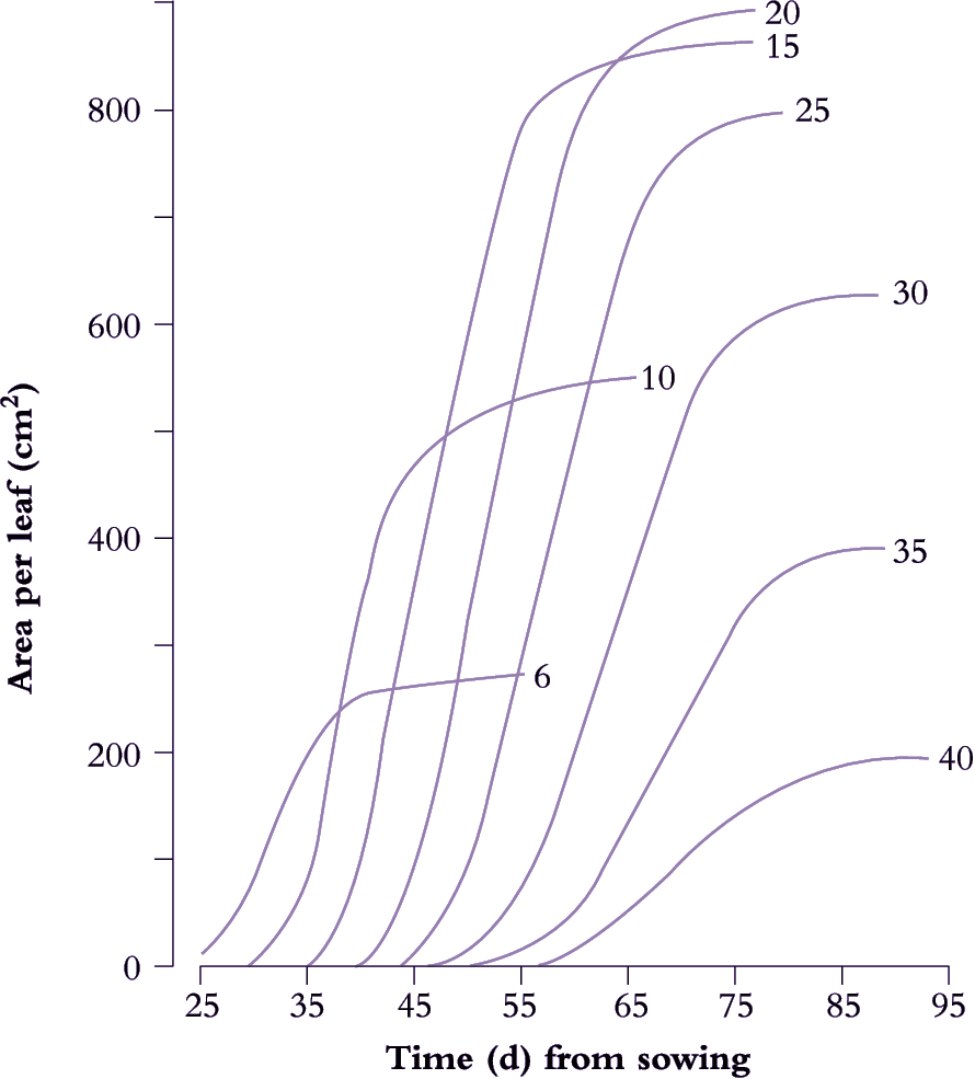
A determinate plant with large leaves such as sunflower (Figure 6.6) provides a typical example. Leaf area is shown as a function of time for eight nodes selected between node 6 and node 40. Final leaf area was greatest at node 20, but daily rates of expansion were uniform for leaves between nodes 10 and 25. Thus at any time between days 35 to 65, the daily rate of expansion of any leaf was the same. Slowest growth and smallest final size was recorded for node 40, adjacent to the terminal inflorescence.

Growth curves for monocots leaves are very similar, in that there is a period of several days during which the leaf has a constant rate of area expansion. Increases in leaf areas of cereals and other monocots are easier to measure than dicots as they grow only in length and not width, for the reason explained below.  

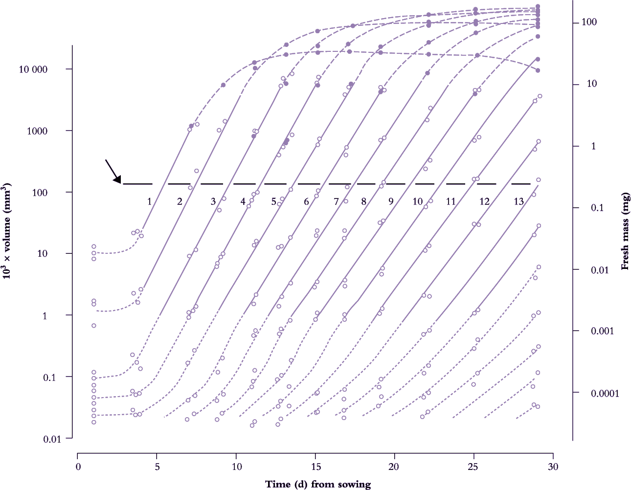
Frequency of leaf initiation can be inferred from a more comprehensive family of such curves where early exponential growth in area for each successive leaf is recorded and plotted as log10 area versus time. This results in a near-parallel set of lines which intersect an arbitrary abscissa (Figure 6.7). Each time interval between successive points of intersection on this abscissa is a ‘phyllochron’ and denotes the time interval between comparable stages in the development of successive leaves. This index is easily inferred from the time elapsed between successive lines on a semi-log plot (Figure 6.7). Cumulative phyllochrons serve as an indicator of a plant’s physiological age in the same way as days after germination represent chronological age.

Fig6.7.png

Figure 6.7. Leaves of subterranean clover achieve a 10-million-fold increase in size from primordium to final area (volume of primordia shown as dotted lines; leaf fresh mass shown as solid lines). Successive leaves are initiated and enlarge in a beautifully coordinated fashion revealed here as a family of straight lines on a semi-log plot. Intervals along an arbitrary abscissa (arrow at 100 × 10-3 mm3) that intersects theses lines represent time elapsed (about 1.8 d) between attainment of a given development status by successive leaves (phyllochron). Full-sized leaves exceed about 100 mm3 in volume. Based on Williams (1975) J Aust Inst Agric Sci 41, 18-26

Fig6.8.png

Figure 6.8. Leaves of cucumber (node 2 on plants in growth cabinets) show an approximately sigmoidal increase in area with time (broken lines) where final size and cell number vary with daily irradiance (0.6, 1.9 or 4.4 MJ m-2 d-1). During an initial exponential phase in area growth, cell number per leaf (solid lines) also increases exponentially. The slope of a semi-log plot (hence relative rate of cell division) is higher under stronger irradiance. Cell number per leaf approaches asymptote as the rate of leaf area increase becomes linear.  Based on Milthorpe and Newton (1963) J Exp Bot 14, 483-495

(b) Developmental stages of leaf expansion

Leaves are first discernible as tiny primordia which are initiated by meristems in accord with a genetically programmed developmental morphology. They undergo extensive cycles of cell division (peak doubling time about 0.5 d). Leaf growth is anatomically different in grasses (monocotyledonous species) and broad-leafed (dicotyledonous) plants.

Primordia of broad-leafed plants undergo extensive cycles of cell division and enlargement to form recognisable leaves with petioles that elongate and lamina that unfold and expand. Lamina expansion follows a coordinated pattern of further cell division and cell enlargement that is under genetic control but modified by the environment, particularly light. Early growth of the leaf is driven primarily by cell division, and cell number per leaf increases exponentially prior to unfolding. Cell division can continue well into the expansion phase of leaf growth, so that up to 90% of cells in a mature dicot leaf can have originated after unfolding. Cell division finishes about the time the leaf enters its period of linear rate of area expansion, so this period of maximum leaf expansion rate is due to expansion of pre-formed cells.

Primordia of grasses and other monocotyledonous species are hidden from view. All phases of cell growth occur at the base of the leaves which are usually not exposed to the environment. Cell division is confined to basal meristems which give rise to files of cells and a linear zone of cell expansion and differentiation. The emerging blade therefore is composed of cells that are fully expanded, and the elongation of that leaf takes place by addition of fully expanded cells from below.

Fig6.9.png

Figure 6.9. Area of individual leaves on cucumber (Cucumis sativus) responds to daily irradiance and reaches a maximum above about 2.5 MJ m-2 d-1. Area increase (node 2 in this example) is due to greater cell number under stronger irradiance. Mean size of mesophyll cells is little affected and has no influence on area of individual leaves. Based on Newton (1963) J Exp Bot 14, 458-482

(c) Effects of light on leaf development

Light is the main variable affecting leaf growth rate, both the rate of leaf area expansion, final size, as well as cell shape as mentioned in the previous section.

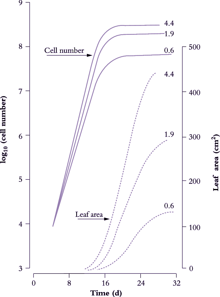
Figure 6.8 shows the effect of light level on the rate of leaf area expansion in a cucumber leaf. As in all dicot leaves, the rate of lamina expansion is determined largely by the number of cells produced, with final cell area being unaffected (Figure 6.9). Rate of cell division during this early phase is increased by irradiance, so that potential size of these cucumber leaves at maturity is also enhanced. The upper curves in Figure 6.8 (highest irradiance), cell number per lamina reaches a plateau around 20 d, but area continues to increase to at least 30 d. Expansion of existing cells is largely responsible for lamina expansion between 20 and 30 d after sowing.

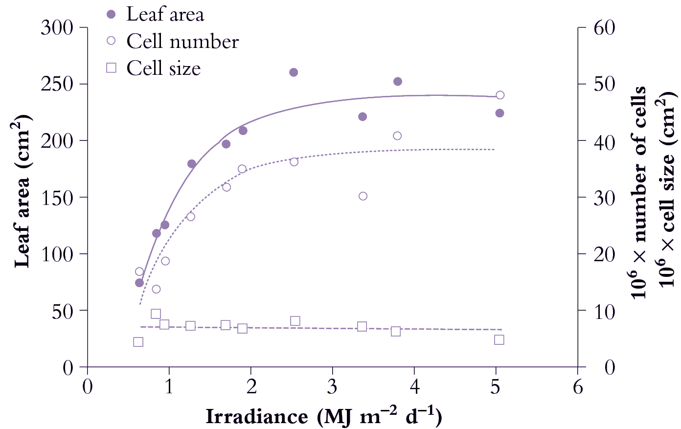
Figure 6.9 shows the effect of a range of light levels on final leaf area, and shows that area is strongly dependent on light level up to 2 MJ m-2 d-1, and that the increased area has been achieved by more cells rather than larger cells.

A similar light response curve would be shown by monocot leaves, and with similar contributions from cell number versus cell size. The difference between monocots and dicots is that the cell number is determined in the basal meristematic zone, before the lamina emerges. This zone is not exposed to the light environment, so cell division activity in monocots is controlled by substrates or signals arising in the older expanded leaves.

 (d) Leaf development and photosynthesis

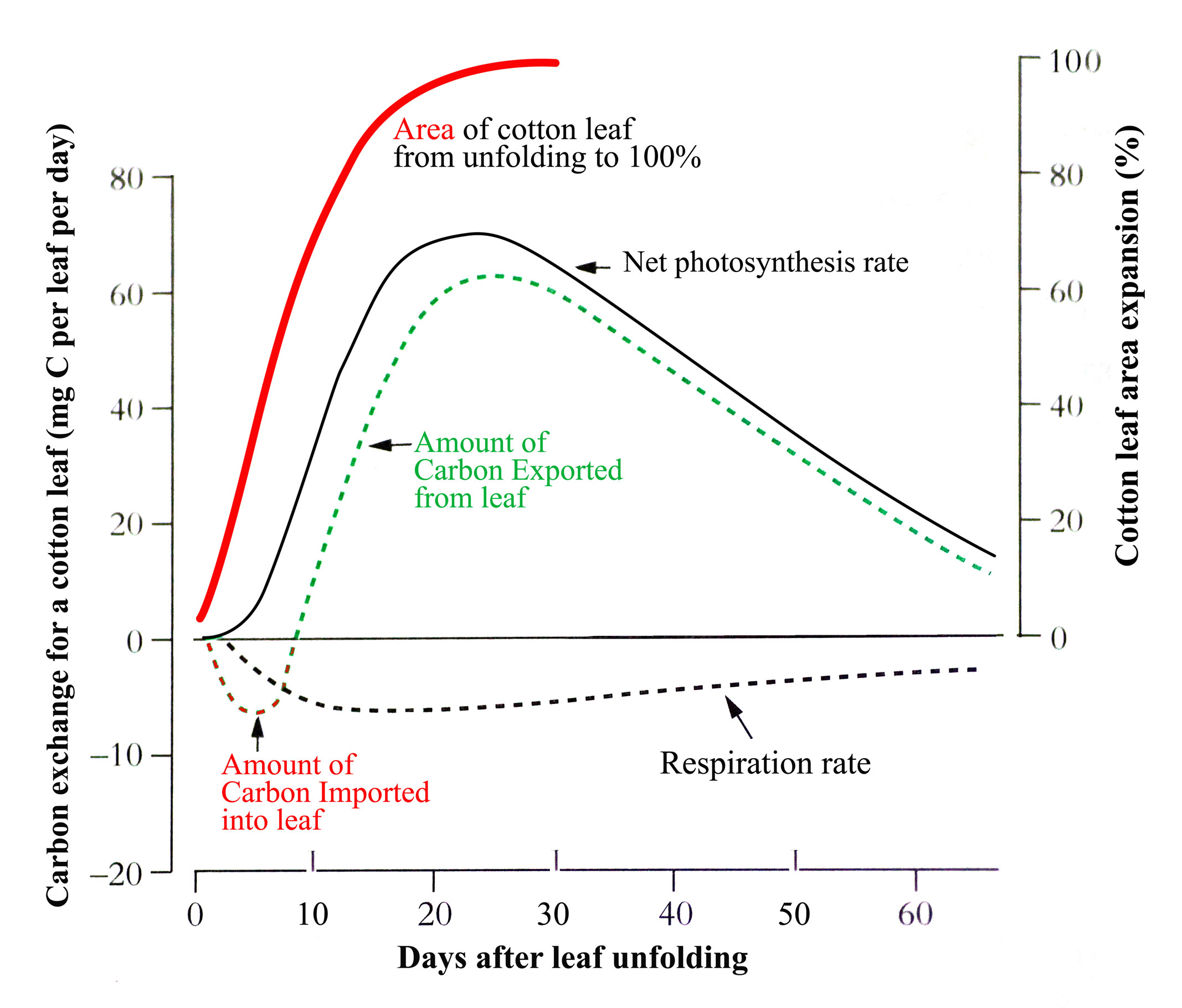
When dicotyledonous leaves are very young and first unfold they have low rates of net photosynthesis (expressed per unit area) so have to import carbon from other leaves to support their growth. But as they expand their rates increase rapidly such that within a few days they can assimilate all their own carbon requirements and export excess (Figure 6.10).

Fig6.10.png

Figure 6.10. Change in net photosynthesis rate as a cotton leaf unfolds, expands, reaches maximum area and ages. An initial phase of carbon import helps sustain early expansion but by the time the leaf is 70% of its final area it is self sufficient for carbon and exporting excess. From Constable and Rawson (1980) Aust J Plant Physiol 7, 89-100 and 539-553

In the example for cotton in the figure, this self-sufficiency occurs when the leaf is about 70% of its final area. Typically, net photosynthesis rate will reach a maximum before the leaf has fully expanded though this can range from 25 to 100% of final area across species. Photosynthesis rate will then remain at that maximum or start to decline with further leaf expansion before leaf aging, lessening requirement for the carbon produced, and environmental factors accelerate the decline. Because the amount of carbon produced by a leaf is the product of two largely independent variables, its photosynthesis rate x its area, leaf carbon production can continue to increase while photosynthesis rate is stable or even declining.

Monocotyledonous leaves grow from their base where the very young expanding parts of the leaf are fully enclosed inside a sheath created by the surrounding leaf bases. The emerged parts of the leaf blade are already approaching full expansion as they emerge from the sheath and unroll. Photosynthesis rates of those exposed parts are already close to their maximum. Once the whole blade is exposed, photosynthesis rate and leaf carbon production follow plateau and declining patterns similar to those described for dicots though magnitude and duration differ amongst species and environments.

When doing experiments that investigate the effects of environmental treatments on photosynthesis, it is important bear in mind the continuous progression in photosynthesis rate between growing, recently fully expanded and aging leaves. Leaves should be compared that are of equivalent age and stage of development, particularly if single leaves are being measured to represent a whole plant or a breeding line. If the eventual aim of the experiment is to compare or select for carbon production, the area of the leaf must also be known since photosynthesis rate and fully expanded area of a leaf are not linked. Leaves of some dicotyledonous species take a few days to reach full expansion while others take weeks.

6.3.2 - Root:shoot ratios

Roots, stems and leaves are functionally interdependent and these three systems maintain a dynamic balance in biomass which reflects relative abundance of above-ground resources (light and CO2) compared with root-zone resources (water and nutrients) (Poorter et al. 2012). Whole-plant growth rate and summary measures such as root:shoot ratio are thus an outcome of developmental stage and of environmental influences.

Change in root:shoot ratio during a plant’s life cycle is part of an intrinsic ontogeny, but growth rates of roots and shoots continually adjust to resource availability with photoassimilate (hence biomass). In herbaceous plants, root:shoot ratios typically decrease with age (size) due to sustained investment of carbon in above-ground structures (root crops would be a notable exception). Developmental morphology is inherent, but expression of a given genotype will vary in response to growing conditions (hence phenotypic plasticity).

Irradiance is a case in point where shoot growth takes priority in low light, whereas root growth can be favoured under strong light. For example, Evans and Hughes (1961) grew Impatiens parviflora at five light levels and demonstrated a steady increase in root mass relative to whole-plant mass (root mass ratio) from 7% to 100% full sun. Stem mass ratio showed the opposite sequence. Leaf mass ratio increased somewhat at low light, but increased SLA was far more important for maintenance of whole-plant RGR in this shade-adapted species.

If light effects on root:shoot ratio are translated via photosynthesis, then CO2 should interact with irradiance on root:shoot ratio because carbon assimilation would be maintained by a more modest investment in shoots exposed to elevated CO2Chrysanthemum morifolium behaved this way for Hughes and Cockshull (1971), returning a higher NAR due to CO2 enrichment under growth cabinet conditions despite lower LAR which was in turn due to smaller leaf weight ratio. Adjustment in SLA exceeded that of leaf weight ratio, and so carried more significance for growth responses to irradiance × CO2.

Consistent with shoot response to above-ground conditions, root biomass is influenced by below-ground conditions where low availability of either water or nutrients commonly leads to greater root:shoot ratio. For example, white clover (Trifolium repens) growing on a phosphorus-rich medium increased root:shoot ratio from 0.39 to 0.47 in response to moisture stress; and from 0.31 to 0.52 when moisture stress was imposed in combination with lower phosphorus (see Table 1 in Davidson 1969b). A positive interaction between low phosphorus and low water on root:shoot ratio was also evident in perennial ryegrass (Lolium perenne) grown on high nitrogen. In that case, root:shoot ratio increased from 0.82 to 3.44 in response to moisture stress when plants were grown on low phosphorus in combination with high nitrogen.

Adding to this nutrient × drought interaction, a genotype × phosphorus effect on root:shoot ratio has been demonstrated by Chapin et al. (1989) for wild and cultivated species of Hordeum. Weedy barleygrass (H. leporinum and H. glaucum) was especially responsive, root : shoot ratio increasing from about 0.75 to 1.5 over 21 d on low phosphorus. By contrast, cultivated barley (H. vulgare) remained between 0.5 and 0.75 over this same period. Held on high phosphorus, all species expressed comparable root:shoot ratios which declined from around 0.55 to about 0.35 over 21 d. High root:shoot ratios on low phosphorus in weedy accessions would have conferred a selective advantage for whole-plant growth under those conditions, thus contributing to their success as weeds.

Even stronger responses to phosphorus nutrition have been reported for soybean (Fredeen et al. 1989) where plants on low phosphorus (10 µM KH2PO4) invested biomass almost equally between roots and shoots, whereas plants on high phosphorus (200 µM KH2PO4) invested almost five times more biomass in shoots than in roots (daily irradiance was about 30 mol quanta m–2 d–1 and would have been conducive to rapid growth).

Root:shoot ratios are thus indicative of plant response to growing conditions, but ratios are not a definitive measure because values change as plants grow. Trees in a plantation forest would show a progressive reduction in root:shoot ratio, and especially after canopy closure where a steady increase in stem biomass contrasts with biomass turnover of canopy and roots and thus predominates in determining root:shoot ratio.

Broad generalisations are that root:shoot ratio increases with nutrient deficiency and moisture stress or under elevated CO2, but decreases in strong light. Too often, however, reports of treatment effects on root:shoot ratio have can overlooked differences in developmental ontogeny or size, and real responses may be obscured. Allometry then becomes a preferred alternative where repeated measurements of size or mass provide an unambiguous picture of carbon allocation.

6.3.3 - Allometry

During whole-plant growth in a stable environment, roots and shoots maintain a dynamic balance such that 

\[y=bx^k \tag{6.17}\]

Where y is root biomass and x is shoot biomass. More generally, x and y can be any two parts of the same organism that are growing differentially with respect to each other, but root–shoot relations are the most common candidate in such analyses of plant growth.

The allometric equation \(y=bx^k\)  (Equation 6.17) was formalised by Huxley (1924) and can be ln transformed to become

\[\text{ln } y= \text{ln }b + k\text{ln }x \tag{6.18}\]

Fig 6.11.png

Figure 6.11. Seedlings of Eucalyptus grandis growing in aeroponic culture on five different nitrogen treatments show a strict allometry between root (Wr) and leaf growth (Wf) (a) as well as between stem (Ws) and leaf growth (b). With all other nutrient elements non-limiting, nitrogen was supplied at five relative addition rates (d-1), namely 0.12 (open circles), 0.10 (solid circles), 0.08 (open triangles), 0.06 (solid triangles) and 0.04 (open square). Root:leaf allometry in seedlings on the lowest relative addition rate (plant [N] 10 mg g-1) shows a similar slope but a higher intercept compared with plants maintained continuously on the highest rate (plant [N] 35.5 mg g-1). Stem:leaf allometry (b) was highly conserved regardless of N addition rate with a slope (k) of 1.261 reflecting a steady commitment to stem growth over leaf growth in these tree seedlings. Based on Cromer and Jarvis (1990) Aust J Plant Physiol 20, 83-98

This formulation enables a straight-line plot of ln y as a function of ln x with slope k  (i.e. the allometric coefficient) and intercept ln b. This empirical model does not explain the nature of growth controls between roots and shoots but does offer a simple description which is not confounded by plant size. Moreover, any departure from a particular root : shoot relationship is immediately obvious, and sources of variation in root : shoot ratio can be resolved into starting conditions (differences in intercept, ln b) versus biomass partitioning during growth (differences in slope, k).

Leaf, stem and root growth under controlled conditions in Eucalyptus grandis seedlings demonstrate such application (Figure 6.11). Nitrogen input in nutrient spray chambers was used as a driving variable for growth where five relative addition rates generated a wide range in whole-plant RGR (from 0.039 d–1  0n lowest to 0.111 d–1 on highest rate).

Data from all treatments and harvests were pooled to reveal a strict allometric relationship between root and leaf growth (Figure 6.11) with a nitrogen effect on intercept but not slope. Nitrogen nutrition had influenced biomass allocation to the extent that low addition rate had initially promoted root growth relative to leaves (hence higher intercept), but subsequent to this early adjustment, and once growth had stabilised, biomass allocation to roots and leaves maintained a constant relationship irrespective of addition rate. In this case k = 0.982, indicating a net bias towards leaf growth over root growth — a ‘net bias’ because carbon loss via excretion, root renewal and respiration was not measured so that more photoassimilate would have been allocated to roots than was fixed in biomass.

Stem and leaf biomass also maintained a strict allometric relationship (Figure 6.11) where k = 1.261. A value for k greater than unity implies a consistent bias towards stem growth relative to canopy growth, as would be expected in a eucalypt with a high rate of stem growth (and favoured in plantation forestry). Significantly, nitrogen treatment was without effect on either intercept or slope (Figure 6.11) and emphasises the highly conserved relationship between leaves and stem in these seedlings.

Fig 6.12.png

Figure 6.12. Root:shoot allometry in Italian reygrass (Lolium multiflorum) shows an abrupt change with flowering (log-log plot). A change in allometric coefficient (k) for this species from 1.121 to 0.553 indicates a shift in biomass allocation from root growth towards shoot growth following emergence of inflorescences. Mean values for k during vegetative cf. Reproductive phase from several accompanying species were 1.145 and 0.627 respectively. Based on Troughton (1956) J Brit Grassland Soc 11, 56-65

Developmental events also influence allometry and Italian ryegrass (Lolium multiflorum) provides a nice example (Figure 6.12) where a log–log plot of root mass as a function of shoot mass showed an abrupt change in slope when flowering occurred. In that case, k decreased from 1.121 to 0.553, and although shoot dry mass was about 10 times root biomass, a change in allometry was clearly evident.