14.2 - Growth and development responses to temperature

Updated by John F Angus and Howard M Rawson, CSIRO Plant Industry, Canberra

Plants can be classified in their temperature responses into broad groups. One group is defined by sensitivity to low temperature: ‘chilling-sensitive’ species are unable to grow, and often suffer visible damage, below 10–15°C and ‘chilling-tolerant’ species are able to grow down to 0°C and able to survive below this temperature.  Within each group, important temperature-sensitive processes are leaf expansion and stem elongation, both of which depend on cell expansion before the cell walls harden.

Another division is based on differences in the pathway of CO2 fixation during photosynthesis, where species in which initial fixation occurs via Rubisco and the photosynthetic carbon reduction cycle are designated C3 species and species in which initial fixation occurs via phosphoenolpyruvate (PEP) carboxylase and the four-carbon dicarboxylic acid pathway are designated C4 species. C4 species include maize and sorghum and such species have high optimum temperatures (≥30°C) for growth. Most C4 plants are also chilling sensitive (Section 14.4). C3 species, on the other hand, show considerable variation in their optimum growth temperature, which can range from close to 30°C in rice to less than 10°C in some alpine species, and they also include a wide range of both chilling-sensitive and chilling-tolerant plants.

14.2.1 - Plant variation in sensitivity to temperature

At any given stage of development, it is possible to define the minimum temperature below which a plant will not grow, suboptimal temperatures where a further increase in temperature will result in increased growth, optimal temperatures when growth is at its maximum, supraoptimal temperatures where a decrease in temperature will result in increased growth and the maximum temperature above which a plant will stop growing. Sustained temperatures beyond this range will be lethal.

Temperature is an important factor in controlling changes in growth and development from germination, through vegetative growth to floral initiation and reproductive growth. Not all stages of development, or different physiological processes, are equally sensitive to temperature. For example, the stage of pollen meiosis during anther development in rice is particularly sensitive to low temperature extremes, whereas in wheat it is less so. Variation in temperature tolerance is also evident within single plants as well as between genotypes. Young actively growing tissues are generally more sensitive to temperature variation than mature tissues and dormant tissues such as buds and seeds can often survive quite extreme temperatures. Frost tolerance in apple is greatest in the stem and then follows a sequence of decreasing tolerance from the mature leaf to the young leaf and floral parts, with the ovary, style and stigma of flowers being least tolerant of frost.

Variation in temperature sensitivity between tissues and physiological processes is also seen in sorghum, a subtropical C4 species. Frost damage occurs to green tissue below –1°C, there is poor seed germination below 6°C, chlorophyll destruction occurs in mature green tissue under high light at 10°C, there is poor pollen development below 13°C and chlorophyll formation in young developing leaves is inhibited at temperatures below 16.5°C (Bagnall 1982).

Fig14.7.png

Figure 14.7. Temperature effects on growth can be viewed in relation to either rate of organ production or the final size attained. Size results from both rate and duration of growth, and there are many examples where organ size is reduced at high temperature because rate of growth cannot compensate for a reduced duration of growth. This is illustrated for wheat (a temperate cereal) and rice (a subtropical cereal). At low temperature wheat has a much larger grain than rice, but rice has a much more stable grain size than wheat in relation to temperature and at 30°C grain size in the two species is very similar. (Based on Tashiro and Wardlaw 1989)

Temperature effects on growth can be viewed in terms of rate multiplied by duration of growth where individual components have different temperature optima (Figure 14.7). As temperature increases within a plant’s dynamic range, duration of growth decreases but rate of growth increases. As a consequence, organ size at maturity may change very little in response to temperature despite variation in growth rate. As temperatures are raised further, an increased rate of growth is no longer able to compensate for a reduction in duration, and the final mass (or volume) of a given organ at maturity is reduced. This is providing that soil water can be maintained during this period. This response can be seen in a range of tissues including leaves, stems and fruits (and seeds). A smaller organ size at maturity due to high temperature is usually associated with smaller cells rather than a change in cell number.

14.2.2 - Thermal time and crop development

As already described, the time taken for plants and their organs to develop within their dynamic temperature range decreases as temperature increases. This was first quantified in the eighteenth century when the French physiologist Reaumur showed that grapes growing in different regions and seasons ripened when the accumulated daily temperature, ti , reached a (fairly) constant value, k, which is known as day degrees, heat units or heatsum. In equation (1) daily temperature is the mean of maximum and minimum temperatures, the subscript i refers to days and the summation was from winter until grape ripening. The units are °C.d.

\[\displaystyle\sum\limits_{winter}^{ripening} t_i=k \tag{14.1}\]

The system of accumulating temperature in this way is known as thermal time and can be applied to the life cycle of a plant or organ, or a phase of a plant’s development such as the seed-filling phase or the expansion of a single leaf.

One weakness of this system is that temperature accumulates above 0°C while in reality, for many species, development stops at temperatures well above freezing.  Instead of accumulating temperatures above 0°C, thermal time systems now use a base or threshold temperature, tbase, which varies with species and is estimated as the value that provides the most constant value of k. Using this system, heat sum is calculated from daily temperatures above tbase , as indicated by the subscript + in equation 2

\[\displaystyle\sum\limits_{finish}^{start} (t_i-t_{base})_{+}  =k \tag{14.2}\]

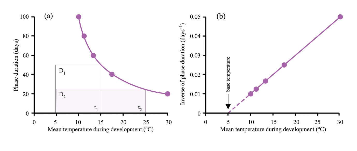
The thermal time system can be simplified providing no daily temperature during a phase falls below tbase.  An example of the simplified system appears as a graph of duration of a phase, D, versus the mean temperature of the phase, ť (Figure 14.8a).  This line is defined by the duration of the phase, D, and the mean temperature of the whole phase above the base temperature, ť-tbase.  The product of these variables is the heatsum, k (equation 3).

\[D(t-t_{base})=k \tag{14.3}\]

Fig14.8.jpg

Figure 14.8. Duration of a phase in a plant’s life cycle, measured as time, decreases as mean temperature increases. For many plants, duration, when measured as thermal units, becomes a constant value. This thermal duration is called a heat sum, heat units or day degrees. It is calculated as the product of time duration and the mean temperature of the phase above a suitable base temperature. The base is 5°C in this graphical example that represents the temperature response of the phase from seedling emergence to flowering (anthesis) of a temperate plant such as wheat. The wheat developmental pattern is shown in (a) as a rectangular hyperbola (purple curve) in which the areas of the rectangles are equal. Expressing the same wheat data as the inverse of time duration against mean temperature (b) produces a straight line. The slope of the straight line is the inverse of the heat sum and the intercept on the x-axis is the base temperature.

Figure 14.8 shows the effect of temperature on phase duration from seedling emergence to flowering (anthesis). The curve in Figure 14.8a is a rectangular hyperbola, meaning that the areas of rectangles defined by the graph are constant, so in the examples \(D_1(t_1'-t_{base})=D_2(t_2'-t_{base})\). For example a duration of 100 days at a mean temperature of 10°C represents a heat sum of 500 °C.d above a base temperature of 5°C i.e. 100(10-5) = 500 °C.d.  The relationship can be linearised by plotting the inverse of duration 1/D against mean temperature (Figure 14.8b). 1/D is defined as the mean rate of development, with units of day-1, and is equivalent to the proportion of development per day (equation 4).

\[\frac{1}{D}=\frac{1}{k}(t'-t_{base})_{+} \tag{14.4}\]

Extrapolation of the line to the x-axis provides an estimate of tbase and the slope of the line, 1/k, is the heatsum.  The advantage of plotting results in this way is that it provides a test of whether the thermal time system works for the data. 

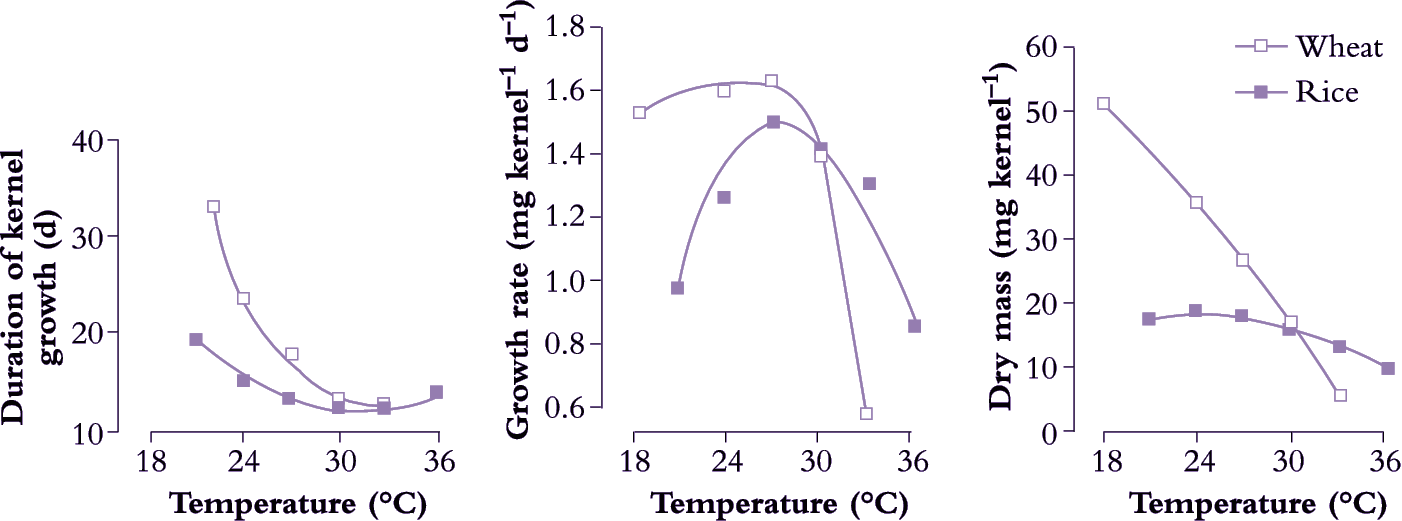
According to this example for wheat, a 2°C warming above a mean of 15°C would reduce the number of days to anthesis from 50 to ~42(500 °C.d / (15°C - 5°C) = 50 days and 500 °C.d / (17°C - 5°C) = 41.7 days).  Reduced duration can mean less crop growth because of fewer days for intercepting solar radiation and photosynthesis. 

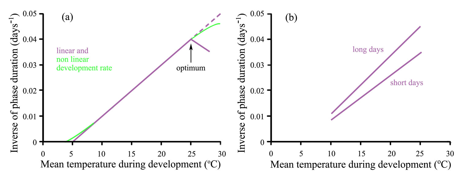
Rate of development is not always linearly related to mean temperature (Figure 14.9a).  At high temperatures the development rate of some plant phases decreases, showing a clear optimum temperature (arrowed).  This cardinal temperature along with the base temperature, defines the boundary of the dynamic temperature range for the phase, organ or species.  An optimum temperature is more likely to appear when plants are exposed to high temperature when light levels are relatively low.  Rate of development is affected by both temperature and photoperiod in photoperiod-sensitive species. So while development responses remain linearly related to temperature the slopes change with photoperiod; a long-day plant develops more rapidly in long days than in short days (Figure 14.9b).

Fig14.9.jpg

Figure. 14.9. Exceptions to the simple thermal time system shown in Figure 14.8. At temperatures close to the base temperature and at high temperatures development may diverge from a linear response of development rate to temperature (shown in (a) as the green departures from the purple straight line). In some species and phases there is a reduced development rate with higher temperature, shown in (a) by the purple line declining beyond the optimum). A long-day plant shows more rapid development in long days than short days over a wide range of temperatures (b).  Short-day plants show the reverse response. Based on Angus et al. (1981).

Thermal time can be used to predict crop development and the stages when herbicides, insecticides and fertiliser should be applied.  This is useful for farmers who manage crops over distances of hundreds of kilometres and need to visit them at a particular stage of development.  Thermal time can also be used to back-calculate the best sowing date to minimise the risk of frost or excessive heat damage at sensitive stages of development.

Fig14.10.jpg

Figure 14.10. Spreadsheet to calculate heatsum from daily maximum and minimum temperatures and a base temperature. Daily mean temperatures below the base do not contribute to heatsum, as shown by the equation in cell G9.

The dynamic ranges of temperatures for subtropical and tropical species are much higher than for this example of temperate wheat.  Consequently the base temperature will be higher and the heatsum different.  Nevertheless the method for calculating thermal time is similar. 

Practical Notes: It is easy to calculate heatsums from temperature data that you measure yourself or download from the internet. Figure 14.10 is a spreadsheet showing a week’s accumulation of heatsums using different base temperatures. When collecting temperature data, remember to shade the thermometer, allow free air circulation and install it at the standard height for your region (1.2 m above ground in Australia).  To test the relationship between heatsum and phasic development you can record development of a phase of plant development in several environments by growing plants at different times of year or in different locations. For that, you need to record on your temperature spreadsheet the date of the start of the chosen phase (maybe the sowing date) and the date of the end of the phase (maybe flowering). Work out the thermal time for each day of the phase like in Figure 14.10, and add all sums together to produce the heatsum for the phase. Compare that result with data you collect from other planting dates. Are the heatsums the same despite different temperatures? If you calculate the mean temperature for the phase on your spreadsheet and the number of days from start to finish of the phase you can graph your combined data like in Figure 14.8. If you have enough sowing dates you will be able to work out the real base temperature for that phase of the chosen species.

Some Definitions:

Development refers to the changes in form or ontogeny of plants (and animals) rather than growth, which means the increase of mass.  While normally growth and development are loosely related, it is possible to have growth without development, for example the continuous growth of vegetative buffalo grass, or to have development uncoupled from growth, for example when the flowering date of stunted drought-affected wheat is similar to the flowering date of well-watered wheat.

Phasic development relates to phases in a plant’s life cycle.  For example the phases in the life cycle of an annual crop are vegetative (between seedling emergence and floral initiation), reproductive (between floral initiation and flowering, called anthesis in wheat) and grain filling (between anthesis and physiological maturity)

Phenology is the science of the influence of climate on the occurrence of biological events

14.2.3 - Photothermal Quotient (PTQ) predicts potential crop yield

PTQ is the ratio of solar radiation to mean temperature during a phase of crop development. Nix (1976) proposed that PTQ could be used to predict potential crop yield, i.e. the yield when crop management overcomes the limitations of water deficit or surplus, nutrient deficiency, pests and diseases. Solar radiation is the numerator because it drives photosynthesis.  Temperature is the denominator because increased temperature leads to faster development and so reduces the time available for photosynthesis.

It is more correct to refer to ‘short-wave global radiation’ than solar radiation because ‘global’ here refers to radiation from the whole sky, including diffuse radiation, but excludes the long waves that have no effect on photosynthesis. The units of PTQ are MJ m-2 d-1 °C-1.  In the case of wheat a base temperature of 0°C is acceptable.  For warm season crops such as maize, a base temperature of 10°C should be used.

Evidence for the accuracy of PTQ comes from three examples of wheat.

Fig14.11.jpg

Figure 14.11. (a) Grain numbers per ear in wheat are set by temperature and radiation during the period from floral initiation to flag leaf expansion as shown by transferring plants amongst temperatures throughout the period. Numbers were closely correlated with PTQ (accumulated radiation divided by thermal time for each of the 24 treatments): After Rawson and Bagga 1979. (b) The relation between PTQ and wheat yield in 23 mini-canopies in controlled environments, compiled by Rawson (1988). The correlation between PTQ and grain number in (a) translated to a close correlation between PTQ and yield in (b) because weight per grain is relatively stable in wheat.  (c) The same linear relationship from (b), see equation 5 below, closely predicts potential grain yield at field scales at locations ranging over many degrees of latitude: southern hemisphere data from Peake and Angus (2009). This suggests that basic meteorological data of temperature and radiation is all that is needed to provide first order estimates of potential crop yields at new locations.

Figure 14.11a shows results from plants grown in naturally-lit temperature-controlled glasshouses and batches transferred every four days between different temperatures during the phases prior to ear emergence. The number of grains per ear changed with temperature but was better correlated with PTQ than with thermal time alone or radiation alone.  Since mean kernel weight is stable for a wheat variety when water and nutrition are adequate, a reasonable hypothesis is that grain yield (grain number x kernel weight) would also be related to PTQ. All that is required to estimate likely potential yield for a location would be local radiation and temperature data. Figure 14.11b shows a test of the grain yield – PTQ relationship with data from temperature-controlled glasshouses and growth chambers using mini-crops of wheat grown in different temperature and radiation environments. The regression fitted to these data was

\[\text{YIELD (t ha}^{-1}) = -3.45+9.59 \text{ PTQ} \tag{14.5}\]

Figure 14.11c shows the line from this equation along with data from commercial crops, including a crop from the Canterbury Plains of New Zealand that set the 2010 world yield record of 15.9 t ha-1

The close relationship between the prediction and the data suggests that PTQ can predict potential wheat yield from tropical to cool temperate zones. PTQ therefore provides farmers with a benchmark to assess the yield of their crops. If their yields are well below the benchmark there is scope for improved crop management or genetics.

References

Angus JF, Mackenzie DH, Morton R, Schafer CA (1981). Phasic development in field crops II. Thermal and photoperiodic responses of spring wheat.  Field Crop Res 4: 269-283

Nix HA (1976) Climate and crop productivity in Australia. In Climate and Rice. International Rice Research Institute, Philippines, pp 495-506

Peake AS, Angus JF (2009) Increasing yield of irrigated wheat in Queensland and northern NSW. Goondiwindi Grains Research Update, March 3-4, 2009. Link: http://www.grdc.com.au/Research-and-Development/GRDC-Update-Papers/2009/11/Increasing-Yield-of-Irrigated-Wheat-in-Queensland-and-Northern-NSW

Rawson HM, Bagga AK (1979) Influence of temperature between floral initiation and flag leaf emergence on grain number in wheat. Aust J Plant Physiol 6: 391-400

Rawson HM (1988) Constraints associated with rice–wheat rotations: effects of high temperatures on the development and yield of wheat and practices to reduce deleterious effects. In AR Klatt, ed, Wheat production constraints in tropical environments. International Maize and Wheat Improvement Center (CIMMYT), Mexico DF, pp 44–62 . Link: http://books.google.com.au/books/about/Wheat_Production_Constraints_in_Tropical.html?id=SBnPP4xZg3oC&redir_esc=y

Tashiro T, Wardlaw IF (1989) A comparison of the effect of high temperature on grain development in wheat and rice. Ann Bot 64::59-65