The wall is an intricate network of polymers that, when capable of expanding, is termed the primary wall. The secondary wall is formed underneath the primary wall when it has finished expanding, and is thicker. The secondary wall is elastic and can shrink or swell but not expand irreversibly like the primary wall.

a) Structure of the primary wall – growing cells

Primary walls are composed predominantly of a complex array of polysaccharides (~90%) and some protein (~10%). In all cell types, rigid cellulose microfibrils are embedded in a gel-like matrix of non-cellulosic polysaccharides and pectins. These polysaccharides are intimately associated with one another, both non-covalently and covalently, and often with proteins and lignins. Walls are complex, diverse and dynamic, changing throughout the processes of cell division, growth and differentiation. The types of wall polysaccharides vary depending on the plant species, cell type and developmental stage (Doblin et al. 2010). In some woody tissues, the secondary wall can be very thick and make up more than half the total volume of the cell.

Growing cells are surrounded by thin walls (100 nm or less) that are sufficiently flexible to yield to the hydrostatic forces that drive growth. The primary walls are highly hydrated (~60% of wet weight) and in dicots and gymnosperms consist of a cellulosic network embedded in a matrix of complex polysaccharides, of which xyloglucans and pectic polysaccharides are most abundant (Figure 7.22). Primary walls of most monocots are organised in essentially the same way except glucans and glucuronylarabinoxylans predominate in the matrix phase and may have properties similar to xyloglucans and pectins.

The main wall constituent that allows the primary wall to expand is the gel-like matrix in which the cellulose microfibrils are embedded. Typically consisting of xyloglucans and pectins, attention is increasingly directed toward the pectins because mutant Arabidopsis plants (xxt1 and xxt2) still can grow even though they totally lack xyloglucans (Cavalier et al. 2008). On the other hand, the genes for pectins have proliferated during the evolution of land plants and Arabidopsis has 15 involved in the synthesis of linear pectins, and 10 more that resemble these genes. Some of their mutants are lethal, especially mutants in GAUT1 and GAUT4 that are the major ones coding for enzymes synthesising linear pectins (Caffal et al., 2009). This suggests a central role for the pectins in the wall. The cellulose does not contribute directly to the growth process and instead mostly strengthens the wall. As a polysaccharide consisting of a linear chain of several hundred to many thousands of β(1–4) linked D-glucose units, it spontaneously crystallises in cellulose microfibrils having about 20 cellulose chains assembled into long cables a few nanometers in diameter. These are cross-linked by hydrogen bonds to a matrix of hemicellulose and pectin along with a small amount of structural protein. The microfibrils have a high tensile strength approaching that of steel, and their orientation in the wall determines the shape of the expansion. When laid down in an orientation perpendicular to the long axis of the cell, lateral expansion is inhibited and the wall extends mostly lengthwise. The longitudinal extension stretches the matrix between the microfibrils, spreading the microfibrils apart. The orientation of the microfibrils thus controls cell shape while the matrix controls growth rate.

b) Structure of the secondary wall – fully grown cells

The secondary wall is laid down underneath the primary wall when it has finished expanding, that is, when the cell has stopped growing. The secondary wall is elastic, it can shrink or swell and undergo reversible but not irreversible expansion. In some woody tissues, the secondary wall can be quite thick and be over half the total volume of the cell.

Cells that have ceased enlarging and are required to withstand large compressive forces mature by depositing secondary walls up to several micrometers thick that increase the wall strength and reduce flexibility (Figure 7.23). During secondary wall development cellulose and matrix phase polysaccharides with a lower degree of backbone substitution, such as heteroxylans and heteromannans, are deposited in a highly ordered pattern. Together with the deposition of lignin this results in a dehydration of the wall material, which becomes increasingly hydrophobic in nature. In some cell types, lignin is also deposited throughout the wall during secondary development. Hydrophobic lignins overlie and encrust the cellulose microfibrils and matrix polysaccharides, and can also be covalently complexed with wall polysaccharides (Doblin et al. 2010). The character of these cells controls woodworking properties of stems of trees and can ward off pathogens that might attack the wood.

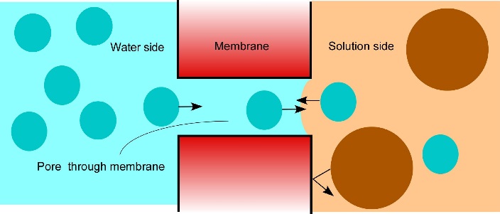
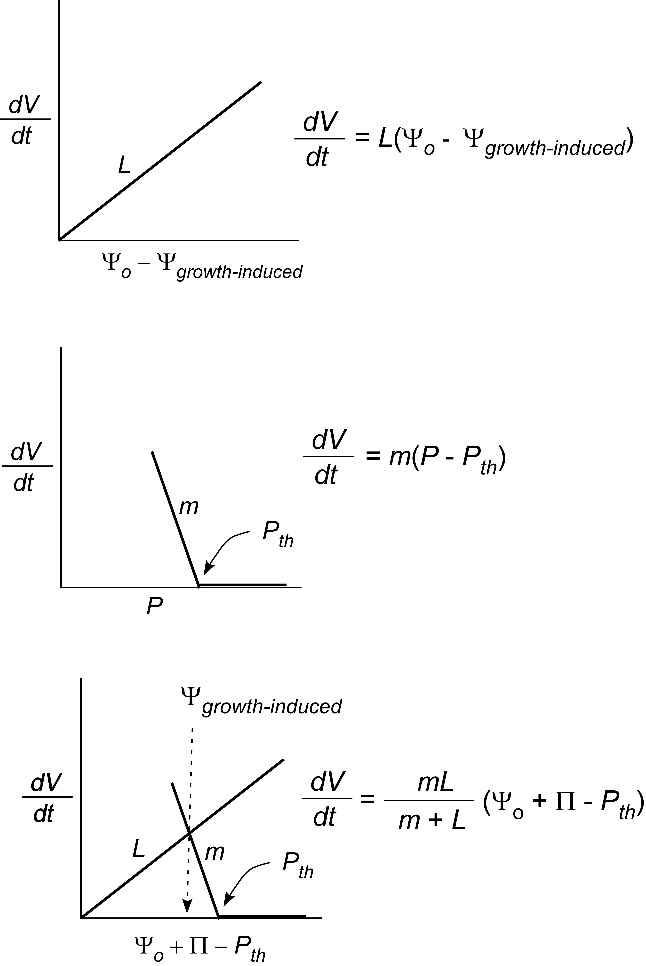
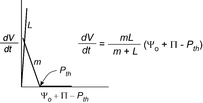
Osmosis makes cell expansion possible. Osmotic concepts were first understood by J. Willard Gibbs (1875-76) and demonstrated experimentally soon thereafter by Wilhelm Pfeffer (1876). Neither of these scientists knew how the process caused growth but Pfeffer (1900) sensed that the critical feature was turgor pressure (P). It is now known that P has to be low enough to create a water potential to bring water into the growing cell while at the same time being high enough to expand the wall. This dual role can be understood from the theoretical basis of osmosis (Figure 7.24).

Osmosis in a constrained compartment like a plant cell causes P to build up inside the cell until it becomes high enough to prevent net water entry. At that stage, the cell is in equilibrium with the solution in its surroundings. Inside the cell, P is the turgor pressure and it can be high (positive pressures of 0.5 MPa are common). Outside of the cell in the wall that is hydraulically connected to the xylem, P can vary considerably and tends to be negative during the day because the xylem water is under tension (negative pressure). The tension in xylem is of course transmitted throughout the apoplast. Bearing this in mind, it is possible to express mathematically the osmotic forces and flows across a membrane as:

\[ \frac{dV}{dt} = AL_{p}[(P_i - P_o) - (\Pi_i - \Pi_o)] \tag{1} \]

where V is the net volume of water moving osmotically across the membrane, \(t\) is the time, \(A\) is the area of the membrane, \(P\) is the pressure, \(\Pi\) is the osmotic effect of the solute concentration, \(L_{p}\) is the hydraulic conductivity of the membrane, and subscripts \(i\) and \(o\) refer to the interior (cytoplasm) and exterior (apoplast) of the cell.

It is important to point out that the water potential is \( \Psi = P – \Pi \) and Eq. 1 simplifies to:

\[ \frac{dV}{dt} = AL_{p} \Delta \Psi \tag{2} \]

where \( \Delta \Psi \) is the water potential difference between the inside and outside of the cell. At equilibrium, \(P\) builds until the net flux is zero and Eq. 1 becomes:

\[ (P_i - P_o) = (\Pi_i - \Pi_o) \tag{3} \]

Let’s see how Eq. 3 fits plant cells whose apoplast is hydraulically connected to the xylem. Starting in the xylem where the solution is very dilute (say \(\Pi_o\) = 0) and the wall solution is under tension (say \(P_o\) = -0.7 MPa), osmosis will move water into the cell as long as the cytoplasm is more concentrated (say \(\Pi_i\) = 1 MPa). As water moves in, \(P_i\) builds inside until it prevents water from entering. Ultimately, the \(P_i\) reaches 0.3 MPa whereupon the cell is equilibrated with its surroundings, as shown in Eq. 3 but expressed numerically in Eq. 4:

\[ 0.3 - (-0.7) = (1 - 0) \tag{4} \]

Notice in Eq. 4 that the P difference across the membrane equals the \(\Pi\) difference across the membrane. In other words, the pressure difference is in equilibrium with the osmotic effect of the solute. Of course, if insufficient water can enter the cell to build its turgor as high as 0.3 MPa, \(P_i\) decreases. If it falls near zero, we sometimes see the leaf “wilting”.

A major advantage of the water potential is that it describes the direction of water movement, taking osmotic properties and pressures into account in one symbol. According to the example above (Eq. 4), the water potential outside of the cell is -0.7 MPa (-0.7 + 0.0). Because outside and inside are in equilibrium, the water potential inside of the cell is also -0.7 MPa (0.3 - 1.0). In both places, \(\Psi\) is a negative number (like temperatures below zero).

Osmosis is the key to water entry into the plant. It not only causes water to enter the cells of the plant but also creates the tension in the xylem transmitted to the cell wall (apoplast) that pulls water through the root from the soil. In fact, this ability to pull water from the soil has to balance transpiration. In other words, water uptake by osmosis is necessary to prevent the plant from drying out. Larger \(\Delta\Pi\) create the potential for greater pull extending out into the soil. Wheat typically contains large \(\Pi_i\) (2.0 to 2.5 MPa) that allows it to obtain water from relatively dry soil. Maize generally has small \(\Pi_i\) (1.2 to 1.8 MPa) that makes it less able to obtain water from dry soil. Maize tends to be less drought tolerant than wheat. The reasons for the \(\Pi_i\) differences are unknown.

These ideas work for osmosis in plant cells that discriminate perfectly between solute and water (water moves through the membrane but solute does not). In healthy cells, most membranes are nearly perfect and negligible solute moves through (solute actually moves through on specific carriers but the amount is negligible osmotically). If solute crosses the membrane, it acts essentially the same as a water molecule, and the osmotic force Π is diminished. Places where this may happen are phloem termini where large amounts of solute are delivered to the developing embryo along with water. Developing grain would be an example. Another place is in air-dry seeds whose membranes have been dehydrated and are leaky to solute until the cells are rehydrated during imbibition, allowing the membranes to re-form.

So far, we have only considered the hydraulic conductivity of membranes of individual cells. Sometimes it might be useful to determine the conductivity of a whole organ such as a root system or leaf. For that an abbreviated form of Eq. 1 is typically used:

\[ \frac{dV}{dt} = L(\Delta\Psi) \tag{5} \]

where \(L\) is called the water conductance of the organ and the definition of the other terms remains unchanged. The reason we cannot use Eq. 2 is that the area for flow is not the plasma membrane of the cell. In effect, \(A\) is undefined and is included in \(L\) but the general principle governing flow is otherwise like that in Eq. 2. As you can see, the bigger the root system the higher the flow and thus \(L\) will tend to get larger as the organ grows.

Plants grow mostly by increasing the size of cells in enlarging regions. For a cell to become larger, the wall becomes irreversibly extended by \(P\). In effect, the wall in a growing cell is constructed so the polymers slip a little at high \(P\). In that situation, as \(P\) builds from osmosis, it never reaches a level where equilibration can occur. Instead, \(P\) can only build enough to cause irreversible slippage (yielding) of the wall and the wall compartment becomes bigger. This can be demonstrated by lowering \(P\). Even if \(P\) decreases as low as zero, the compartment remains bigger than it was.

Typically the \(P\) must be higher than a minimum before yielding occurs. It is possible to express this wall property with an equation similar to Eq. 2. Lockhart (1965) was the first to do so and described cell enlargement for \(P\)-driven growth as:

\[\frac{dV}{dt} = A \phi (P - P_{th}) \tag{6} \]

where \(\phi\) is the wall yielding coefficient, sometimes referred to as wall extensibility (m Pa^–1 s^–1) and \(P_{th}\) is threshold turgor pressure or yield threshold (\(P_{th}\)) above which the cell wall yields. The other terms are defined as before. It is obvious in Eq. 6 that \(P\) must be above \(P_{th}\) in order for the cell to enlarge. Also, as \(\phi\) becomes larger, the cell grows faster.

In tissues instead of individual cells, a similar equation applies because all the cells enlarge in concert. The enlargement of the whole organ is then described by:

\[\frac{dV}{dt} = m (P - P_{th}) \tag{7} \]

where everything is the same as in Eq. 6 except that \(m\) contains the wall yielding attributes for all the enlarging cells as well as the \(A\) term. Examples where this equation applies would be tissues of enlarging stem and root tips, hypocotyls and coleoptiles of geminating seeds, flower buds, and even growing fruits (grapes, tomatoes, maize kernels, etc).

Nevertheless, the inability of \(P\) to build enough for equilibration keeps the cell water potential lower than it otherwise would be. As a result the yielding walls create a lower water potential that is called “growth-induced” because mature cells that do not have such yielding walls (Figure 7.25). The growth-induced \(\Psi\) can move water from the mature cells into the elongating ones if no external supply is available. This probably explains how a stored potato can sprout in a cupboard because the cells in the bud develop yielding walls that create a growth-induced \(\Psi\) that moves water from the mature cells into the sprouts.

Usually the water source is in the soil or xylem (\(\Psi_o\)), and a slight modification to Eq. 5 can show this effect:

\[\frac{dV}{dt} = L (\Psi_o - \Psi_{growth-induced}) \tag{8} \]

Because the cells with yielding walls have turgor that is \(P = \Pi + \Psi_{growth-induced}\) (remember \(\Psi\) is negative), Eq. 7 becomes:

\[\frac{dV}{dt} = m (\Pi + \Psi_{growth-induced} - P_{th}) \tag{9} \]

and solving for \(\Psi_{growth-induced}\) in Eqs 8 and 9 gives:

\[\frac{dV}{dt} = \frac{mL}{m + L} (\Psi_o + \Pi - P_{th}) \tag{10} \]

This shows that growth depends on a water supply function (Eq. 8) and a water demand function (Eq. 7) that can be combined to give Eq. 10. A quick look at this latter expression shows that the growth rate of an organ is determined by the water potential of the supply, the osmotic effect of the solute minus the threshold turgor (which is too low to contribute to the growth rate) multiplied by a coefficient. In other words, the difference in water potential that we’ve seen before in Eq. 5 diminished by the threshold turgor that is inactive in the growth process provides the driving force for growth. When multiplied by the coefficient, \(\frac{mL}{m + L}\), the equation gives the growth rate of the organ.

The reason Eq. 10 is important is that it shows a plant organ grows not only because of the turgor properties of the tissue but also because water moves through all the small cells (\(L\)) of the entire organ. Meristems have dividing cells that are necessarily small. There are many wall and membrane barriers to traverse before water reaches all of the cells and allows them to grow simultaneously at a similar rate. The yielding of the walls controls the growth-induced \(\Psi\) needed for this water. In effect the turgor must be high enough for the walls to yield but low enough to create the growth-induced potential to supply water to the enlarging cells. The supply is often quite far away depending on the anatomy of the meristem and enlarging tissues. Consequently, large distances may be travelled by water for growth and the anatomy plays a large part in the growth rate of the organ.

It is worth looking at the coefficient a little more deeply. If the wall yields easily and m is large (say \(m\) = 10 units and \(L\) = 1 unit), the coefficient is 10/11 and the growth rate is controlled mostly by the ability of water to move into the enlarging tissues. If the reverse occurs (\(m\) = 1, \(L\) = 10), the coefficient is still 10/11 but the growth rate is controlled mostly by the yielding properties of the walls. Therefore, comparing the magnitude of \(m\) and \(L\) is the key to determining whether the demand (\(m\)) or the supply (\(L\)) function dominates the coefficient. A picture of these effects is shown in Figure 7.26 and methods are available for measuring not only \(m\) and \(L\) but also all the other terms in these equations (Boyer et al., 1985).

It is pretty obvious from this behaviour that simply putting water around a tissue creates a system with several interacting factors. The growth rate could be affected not only by \(P\) but also by \(m\), \(L\), \(\Pi\), or \(P_{th}\). In an effort to simplify this system, scientists have sought single cells that could be surrounded by water. From a practical point of view this allows \(P\) and \(m\) to be the main factors controlling growth and minimises the effect of \(L\), as shown in Figure 7.27.

One approach has been to use single algal cells large enough to measure \(P\) and growth (\(\frac{dV}{dt}\)) simultaneously. Chara corallina or Nitella flexilis are candidates because they have cells large enough for the measurements. They are naturally surrounded by fresh or brackish water and have rhizoids resembling roots. Gametes form in structures in the axils of branches analogous to flowers or cones in their land counterparts. In fact, genomic and morphological analyses consider these algae to be among the closest relatives of the progenitors of land plants. In the internode cells of Chara or Nitella, microfibrils are oriented normal to the cell axis and the walls expand mostly in length like many plant tissues (roots, stems, grass leaves).

Using the internodes of these species, \(P\) and growth rate (\(\frac{dV}{dt}\)) can be monitored simultaneously and changed so quickly that \(\Pi\) and \(P_{th}\) remain constant. This allows the \(P\) response to be rigorously determined. Moreover, the walls can be isolated without leaving the medium in which the algae are grown. The same measurements can be repeated without the cytoplasm. This is a great tool for observing the response to \(P\). When the growth of the live cells was compared with that in the isolated walls, they were similar but only for the first hour or so. After that, growth ceased in the walls but continued in the live cells even though the walls and cells had the same \(P\). Something was missing in the isolated wall that was being supplied by the live cells.

Considering that new wall material is supplied by the cytoplasm and missing in the isolated walls, if seemed reasonable to supply new wall constituents as though the cytoplasm had done so. Supplying pectin (a wall polymer) to the growth medium returned the growth rate of isolated walls to the rate in the live cells! This was unexpected but indicated the wall needed a supply of pectin in order to continue growing. The active pectin was a linear unbranched polymer of α-1,4-D-galacturonic acid sometimes with a small amount of rhamnose (usually 1-2%) that is normally synthesised in the cytoplasm and released to the wall by exocytosis. It becomes a prominent member of the wall matrix and forms a gel embedding the cellulose microfibrils.

The pectin gels because calcium ions bind to neighbouring pectin polymers. The cross-bridging forms junction zones with the polymers that are strong enough for the pectin to form a gel solid. The gel gets stronger with more cross-bridges. The new pectin from the cytoplasm removed some of the cross-bridges from the wall, weakening the wall gel and allowing the polymers to slip a little. This action occurred only when \(P\) was above \(P_{th}\), and only when temperatures were warm enough for growth. Figure 7.28 compares the turgor pressure and temperature responses of the live algal cells with those of land plants tissues.

A chemical mechanism has been proposed to account for this behaviour and is called a “calcium pectate cycle” (Figure 7.29). It seems possible that the chemistry might also occur in land plants. As long as pectin, calcium, and sufficient turgor pressure are present, the cycle should occur in pectin-containing walls. Pectins are among the most conserved components of cell walls during plant evolution, and the similarity in pressure and temperature response in these algae and land plants suggests a common mechanism in both. However, despite these intriguing similarities, definitive tests remain for the future.

Expansins

In other experiments a class of cell wall proteins, expansins, are proposed as potential agents for catalysing yielding in vivo (McQueen-Mason 1995). Figure 7.30 shows sharp gradients in growth along the hook of a cucumber hypocotyl that are paralleled by a gradient in extension of these tissues when stretched under acid conditions (Figure 7.30b) but not at neutral pH (Figure 7.30c). When tissues were killed by boiling, extension was blocked (Figure 7.30d). From these results, it seems that hypocotyl extension requires acid pH and non-denatured proteins. However, all the experiments were done in an extensometer with a uni-axial pull substantially less than the multi-axial tension exerted by \(P\). Since growth requires \(P\) above a threshold in order for walls to yield (Eq. 7), it is difficult to interpret this proposal. When greater uni-axial pull was used by Ezaki et al. (2005) to study hypocotyl growth in soybean hypocotyls, pectin chemistry appeared to determine growth rate. In fact, Zhao et al. (2008) give evidence that pectins may be the target of expansin action.

Notice that the growth mechanism in Figure 7.29 is entirely chemical, with no role for enzymes. It is difficult to hypothesize an enzymatic mechanism because of the requirement for \(P\) above a threshold. Enzyme activity is generally unaffected by these pressures and would continue acting regardless of \(P\). What is clear is that the biophysical consequences of instantaneous changes in \(P\) will be followed by a phalanx of biochemical events including wall polymer synthesis and altered gene expression, and rigorous methods will be required to distinguish enzymatic from biophysical hypotheses. For instance, sustained expansion of plant cell walls cannot be explained simply by inexorable wall hydrolysis; if it were, cell walls would weaken to breaking point during growth. The ‘setting’ of long-term cell expansion rates is likely to hinge on biochemical and chemical events underlying wall relaxation and reinforcement.

Cessation of cell wall expansion

Molecular events leading to cessation of wall expansion are even less well understood than those which initiate growth. For example, part of the growing region stops growing when water deficits occur around maize roots (Figure 7.31).

Clearly, the region farthest from the tip has stopped growing but \(P\) remains uniform throughout the zone. \(P\) is lower in the water deficient roots presumably because less water can be absorbed from the water deficient soil. A common view is that sufficient cross-linking develops to limit the extension of the matrix around cellulose microfibrils and prevent further wall expansion. Essentially, when a cell has reached its final dimensions its wall is ‘locked’ into a final, hardened conformation. From the description above, molecules with a specific role in growth cessation are thought to be exocytosed into cell walls, providing either substrates for cross-linkage reactions or enzymes catalysing cross-linkage of pre-existing wall polymers. Identification of cross-linkage reactions have led to a search for their presence in vivo. For example, ferulic acid residues in grass cell walls can cross-link to produce di-ferulic acid and potentially stiffen walls through formation of a polysaccharide-lignin network. Unfortunately, in rice coleoptiles the abundance of the di-ferulic form bore no relation to growth cessation. Also this form of stiffening might be difficult to distinguish from secondary wall deposition.

Secondary cell walls generally form after primary walls have ceased to grow but the familiar rigidity of secondary cell walls (e.g. wood) is mostly viewed as distinct from stiffening of primary walls. Lignification of primary walls commences earlier than once thought and is a possible factor in growth cessation (Müsel et al. 1997). Such a response might be controlled through release of peroxide into walls in much the same way as seen in walls subject to fungal attack. Peroxidase enzymes are candidates for the catalysis of these reactions. Understanding rigidification of this complex matrix of polymers demands input from the disciplines of biology, chemistry and physics. Combining established techniques with novel approaches to the study of individual cells (e.g. Fourier-Transform Infra-red microspectroscopy and the cell pressure probe) will bring new insights to the molecular basis of wall expansion.