Plants grow mostly by increasing the size of cells in enlarging regions. For a cell to become larger, the wall becomes irreversibly extended by \(P\). In effect, the wall in a growing cell is constructed so the polymers slip a little at high \(P\). In that situation, as \(P\) builds from osmosis, it never reaches a level where equilibration can occur. Instead, \(P\) can only build enough to cause irreversible slippage (yielding) of the wall and the wall compartment becomes bigger. This can be demonstrated by lowering \(P\). Even if \(P\) decreases as low as zero, the compartment remains bigger than it was.
Typically the \(P\) must be higher than a minimum before yielding occurs. It is possible to express this wall property with an equation similar to Eq. 2. Lockhart (1965) was the first to do so and described cell enlargement for \(P\)-driven growth as:
\[\frac{dV}{dt} = A \phi (P - P_{th}) \tag{6} \]
where \(\phi\) is the wall yielding coefficient, sometimes referred to as wall extensibility (m Pa–1 s–1) and \(P_{th}\) is threshold turgor pressure or yield threshold (\(P_{th}\)) above which the cell wall yields. The other terms are defined as before. It is obvious in Eq. 6 that \(P\) must be above \(P_{th}\) in order for the cell to enlarge. Also, as \(\phi\) becomes larger, the cell grows faster.
In tissues instead of individual cells, a similar equation applies because all the cells enlarge in concert. The enlargement of the whole organ is then described by:
\[\frac{dV}{dt} = m (P - P_{th}) \tag{7} \]
where everything is the same as in Eq. 6 except that \(m\) contains the wall yielding attributes for all the enlarging cells as well as the \(A\) term. Examples where this equation applies would be tissues of enlarging stem and root tips, hypocotyls and coleoptiles of geminating seeds, flower buds, and even growing fruits (grapes, tomatoes, maize kernels, etc).
Nevertheless, the inability of \(P\) to build enough for equilibration keeps the cell water potential lower than it otherwise would be. As a result the yielding walls create a lower water potential that is called “growth-induced” because mature cells that do not have such yielding walls (Figure 7.25). The growth-induced \(\Psi\) can move water from the mature cells into the elongating ones if no external supply is available. This probably explains how a stored potato can sprout in a cupboard because the cells in the bud develop yielding walls that create a growth-induced \(\Psi\) that moves water from the mature cells into the sprouts.
Usually the water source is in the soil or xylem (\(\Psi_o\)), and a slight modification to Eq. 5 can show this effect:
\[\frac{dV}{dt} = L (\Psi_o - \Psi_{growth-induced}) \tag{8} \]
7.3-Ch-Fig-7.25.jpg
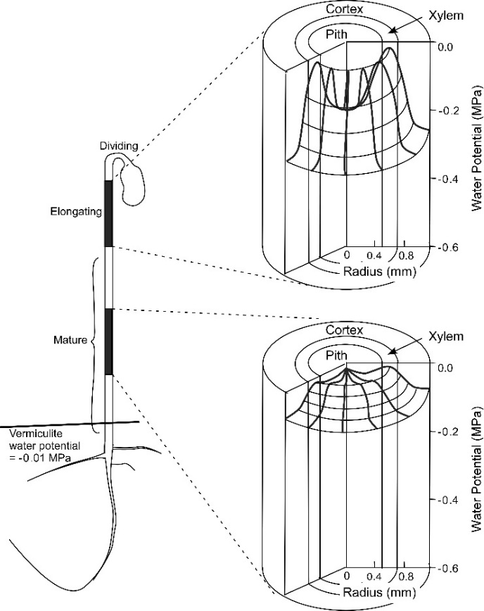
Figure 7.25 Water potential fields (three dimensions) in two regions of soybean hypocotyls growing at about 1.5 mm h-1. Fields show highest water potential in the xylem and lowest in the pith and cortex. Steepest field was in the elongating tissues and is growth-induced because the yielding walls in the elongating cells prevented \(P\) from become as high as in mature cells. The steeper field allows the growing region to extract water from the mature region when other water sources are not available. Fields were directly measured in the same intact plant while transpiration was prevented, using a microcapillary of a pressure probe. (Redrawn from H Nonami and JS Boyer, Plant Physiol 102: 13-19, 1993).
Because the cells with yielding walls have turgor that is \(P = \Pi + \Psi_{growth-induced}\) (remember \(\Psi\) is negative), Eq. 7 becomes:
\[\frac{dV}{dt} = m (\Pi + \Psi_{growth-induced} - P_{th}) \tag{9} \]
and solving for \(\Psi_{growth-induced}\) in Eqs 8 and 9 gives:
\[\frac{dV}{dt} = \frac{mL}{m + L} (\Psi_o + \Pi - P_{th}) \tag{10} \]
This shows that growth depends on a water supply function (Eq. 8) and a water demand function (Eq. 7) that can be combined to give Eq. 10. A quick look at this latter expression shows that the growth rate of an organ is determined by the water potential of the supply, the osmotic effect of the solute minus the threshold turgor (which is too low to contribute to the growth rate) multiplied by a coefficient. In other words, the difference in water potential that we’ve seen before in Eq. 5 diminished by the threshold turgor that is inactive in the growth process provides the driving force for growth. When multiplied by the coefficient, \(\frac{mL}{m + L}\), the equation gives the growth rate of the organ.
7.3-Ch-Fig-7.26.jpg
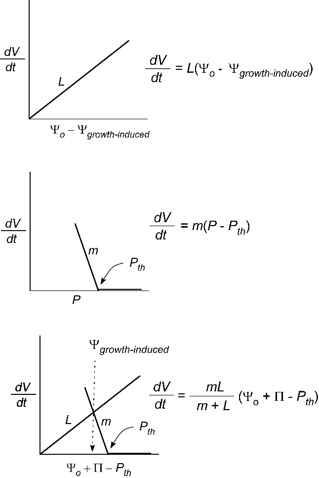
Figure 7.26 Diagram of the steady growth of a plant organ. Water uptake for growth (\(dV/dt\)) is a simple linear function of the conductance (\(L\)) between the water supply (\(\Psi_o\), usually the vascular system) and the average water potential (\(\Psi_{growth-induced}\)) of all the expanding cells in the organ (top of diagram, Eq. 7). In the same organ, the cells have walls that can slip a little (\(m\)) when turgor (\(P\)) is above a threshold (\(P_{th}\)) (middle, Eq. 8). Combining the two relations defines the \(\Psi_{growth-induced}\) and \(P\) for the organ (Eq. 10, bottom). Notice that the \(\Psi_{growth-induced}\) is always lower than the (\(\Psi_o\). Furthermore, the position of \(\Psi_{growth-induced}\) is determined by \(L\) and \(m\). (Diagram courtesy JS Boyer)
It is worth looking at the coefficient a little more deeply. If the wall yields easily and m is large (say \(m\) = 10 units and \(L\) = 1 unit), the coefficient is 10/11 and the growth rate is controlled mostly by the ability of water to move into the enlarging tissues. If the reverse occurs (\(m\) = 1, \(L\) = 10), the coefficient is still 10/11 but the growth rate is controlled mostly by the yielding properties of the walls. Therefore, comparing the magnitude of \(m\) and \(L\) is the key to determining whether the demand (\(m\)) or the supply (\(L\)) function dominates the coefficient. A picture of these effects is shown in Figure 7.26 and methods are available for measuring not only \(m\) and \(L\) but also all the other terms in these equations (Boyer et al., 1985).